
この記事はStan Advent Calendar 2019の17日目の記事になります。今年もエポックメイキングな記事が多い中,この記事では例年に倣って,重箱の隅をつついて行きたいと思います。どうも,RStan界隈のすみっコぐらしです。
brmsパッケージのAdditional response information
ご存知,brmsパッケージでは,一般化線形モデルなどの回帰系のモデルを,Stanを用いて推定することが可能です。brmsパッケージを使ったことがない,そもそも知らないという方は,今すぐ@das_Kinoさんの解説記事を読んでください。今すぐです。最近ですと,馬場真哉 先生の『RとStanではじめるベイズ統計モデリングによるデータ分析入門』の5章にも解説があります。brmsパッケージによって,線形モデルのベイズ推定に対するハードルは随分下がったといえるでしょう。
そんなbrmsパッケージには,ちょっと応用的な応答変数を扱える,Additional response informationという機能があります。brmsパッケージの説明書の”brmsformula”の項に解説がありますが,要するに「brmsのモデルの応答変数に,他の変数との対応関係のような追加の情報を付け加える」という機能で,この記事を書いた時点で,se()関数やweights()関数など,計11種類の関数が実装されています。
使い方は,brmsのモデル式の左辺に,応答変数に続けて”|”演算子と追加情報に関する変数を記述します。例えば,brmsパッケージに含まれるkidneyデータ (腎臓病患者に関するデータ) では,”time”という変数に病気の再発までの時間が,”censored”という変数に”time”が正しく打ち切られたデータなのかどうかの情報が入力されています (Bürkner, 2017※1の例を参考にしています)。
> head(kidney)
  time censored patient recur age    sex disease
1    8        0       1     1  28   male   other
2   23        0       2     1  48 female      GN
3   22        0       3     1  32   male   other
4  447        0       4     1  31 female   other
5   30        0       5     1  10   male   other
6   24        0       6     1  16 female   other
このとき,cens()関数を使って以下のようにモデルを書くことで,反応時間と打ち切りの有無の変数を対応づけることができ,打ち切りの影響を加味したモデルにすることが可能です。
model <- bf(
  time | cens(censored) ~ [任意の予測変数]
)
このAdditional response informationを使うことで,ただでさえ多機能なbrmsパッケージの拡張性がさらに高まります。以下では例として,Bürkner (2019)※2 を参考に,dec()関数を使ったDrift Diffusion Modelによる分析を再現してみましょう。その他の関数でどんなことができるかについては,上述の解説部分をご参照ください。
brmsパッケージでDrift Diffusionモデル
Drift Diffusionモデルは,実験参加者の2値反応と反応時間のデータをもとに,閾値α,反応バイアスβ,ドリフト率δ,非決定時間τの4つのパラメータを推定する認知モデルです。ちょうど,昨日のStanアドカレ記事にDiffusionモデルの素晴らしい解説がありますので,併せてご参照ください。
データとして,diffIRTパッケージに含まれる”rotation”データを用います。Bürkner (2019) のTable 2の形と揃うように整形しています。
#パッケージ読み込み
library(tidyverse)
library(rstan)
library(bayesplot)
library(brms)
library(diffIRT)
#rotationデータ読み込みと整形
data("rotation")

rtt_resp <- data.frame(rotation[,1:10])
rtt_time <- data.frame(rotation[,11:20])

colnames(rtt_resp) <- c("1":"10")
colnames(rtt_time) <- c("1":"10")

rtt_resp$person <- 1:121
rtt_time$person <- 1:121

rtt_resp_new <- gather(rtt_resp,
                       key = "item",
                       value = "resp",
                       "1":"10")

rtt_time_new <- gather(rtt_time,
                       key = "item",
                       value = "time",
                       "1":"10")

rotate_new <- inner_join(rtt_time_new,
                         rtt_resp_new,
                         by = c("item", "person"))

rotate_new <- mutate(rotate_new,
                     rotate = case_when(
                       item == 1 ~ "150",
                       item == 2 ~ "50",
                       item == 3 ~ "100",
                       item == 4 ~ "150",
                       item == 5 ~ "50",
                       item == 6 ~ "100",
                       item == 7 ~ "150",
                       item == 8 ~ "50",
                       item == 9 ~ "150",
                       item == 10 ~ "100"))

rotate_new <- transform(rotate_new,
                        rotate = factor(rotate,
                                        levels = c("50", "100", "150")))

rotate_new <- arrange(rotate_new,
                      person, item)
データはこんな感じです。メンタルローテーションの実験データで,角度を50°,100°,150°傾けた1〜10の刺激があります。”time”の変数は各刺激への反応時間を,”resp”の変数は参加者の反応 (”1”が正答,”0”が誤答) を表します。
> head(rotate_new)
  person item  time resp rotate
1      1    1 4.444    1    150
2      1   10 5.447    1    100
3      1    2 2.328    1     50
4      1    3 3.408    1    100
5      1    4 5.134    1    150
6      1    5 2.653    1     50
分析の目的は,「刺激の角度によってDiffusionモデルのパラメータに違いが見られるか」を検討することです。モデルの記述は以下のようになります。
#呪文(ndtの推定が難しいので切片の初期値を小さく設定しておくらしい)
chains <- 4
inits_drift <- list(temp_ndt_Intercept = -3)
inits_drift <- replicate(chains, inits_drift, simplify = FALSE)

#モデル
#bs=閾値,ndt=非決定時間,bias=反応バイアス
#非決定時間を0.1,バイアスを0.5で固定
DDM_model <- bf(
  time | dec(resp) ~ rotate + (1 |p| person) + (1 |i| item),
  bs ~ rotate + (1 |p| person) + (1 |i| item),
  ndt = 0.1,
  bias = 0.5)
モデル部分でAdditional response informationの1つであるdec()関数を使っています。”dec”は”decision”の略で,応答変数である”time”と,参加者の正答/誤答の情報である”resp”が対応していることを表しています。こうすることで,正答の場合の反応時間と誤答の場合の反応時間を分けた分析ができるというわけです。
モデルの当てはめと結果の出力は以下の通りです。marginal_effects()関数で各パラメータにおける変数”rotate”の主効果を図示しています。
#モデル当てはめ・結果出力
DDM_fit <- brm(DDM_model,
               data = rotate_new,
               family = brmsfamily("wiener", "log", link_bs = "log", link_ndt = "log"),
               chains = chains,
               cores = chains,
               inits = inits_drift,
               init_r = 0.05,
               control = list(adapt_delta = 0.99))

summary(DDM_fit)

marginal_effects(DDM_fit, "rotate", dpar = "mu")
marginal_effects(DDM_fit, "rotate", dpar = "bs")
> summary(DDM_fit)
 Family: wiener
  Links: mu = log; bs = log; ndt = identity; bias = identity
Formula: time | dec(resp) ~ rotate + (1 | p | person) + (1 | i | item)
         bs ~ rotate + (1 | p | person) + (1 | i | item)
         ndt = 0.1
         bias = 0.5
   Data: rotate_new (Number of observations: 1178)
Samples: 4 chains, each with iter = 2000; warmup = 1000; thin = 1;
         total post-warmup samples = 4000

Group-Level Effects:
~item (Number of levels: 10)
                            Estimate Est.Error l-95% CI u-95% CI Rhat Bulk_ESS Tail_ESS
sd(Intercept)                   0.28      0.11     0.15     0.56 1.00     1310     1966
sd(bs_Intercept)                0.07      0.04     0.00     0.17 1.00     1029     1687
cor(Intercept,bs_Intercept)     0.37      0.44    -0.71     0.95 1.00     2370     2515

~person (Number of levels: 121)
                            Estimate Est.Error l-95% CI u-95% CI Rhat Bulk_ESS Tail_ESS
sd(Intercept)                   0.83      0.07     0.71     0.97 1.00      904     1823
sd(bs_Intercept)                0.43      0.04     0.36     0.50 1.00      833     1441
cor(Intercept,bs_Intercept)     0.89      0.03     0.82     0.93 1.00     1189     2286

Population-Level Effects:
             Estimate Est.Error l-95% CI u-95% CI Rhat Bulk_ESS Tail_ESS
Intercept        0.09      0.20    -0.32     0.48 1.00      959     1348
bs_Intercept     1.86      0.07     1.73     2.00 1.00     1080     1862
rotate100       -0.40      0.26    -0.89     0.12 1.00     1210     1611
rotate150       -0.37      0.24    -0.85     0.11 1.00     1096     1463
bs_rotate100    -0.01      0.08    -0.18     0.15 1.00     1822     1840
bs_rotate150    -0.02      0.08    -0.17     0.14 1.00     1730     1828

Samples were drawn using sampling(NUTS). For each parameter, Eff.Sample
is a crude measure of effective sample size, and Rhat is the potential
scale reduction factor on split chains (at convergence, Rhat = 1).
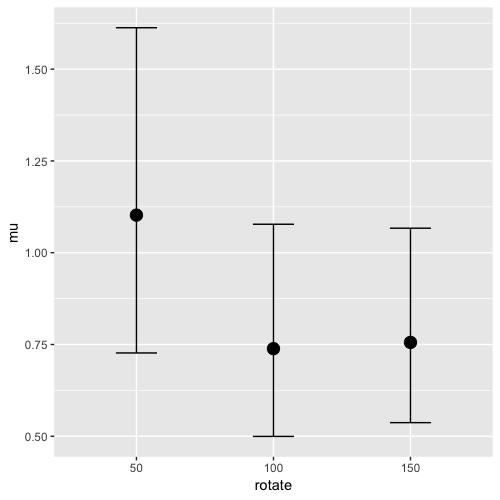
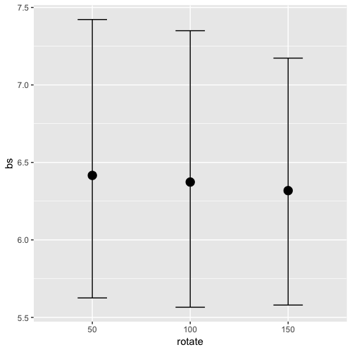
主効果の図を見る限り,ドリフト率δ (mu) は刺激の角度の影響を受けているように見えます。ただし,傾きの95%確信区間が0を跨いでいるので,あまり確かなことは言えません。閾値に関しては,角度による影響はなさそうです。
brmsパッケージは万能ではない
上記の結果を見て,あれ?DDMのパラメータは4つじゃなかった?と思った方もおられるのではと思います。実は,Bürkner自身も論文中で書いているように,brmsを使ったDDMの推定は結構繊細です。自分自身のデータでも色々と試してみましたが,特に非決定時間 (ndt) のパラメータの初期値がなかなか求まらず,推定が始まらないことも多いです。今回の分析でも,非決定時間とバイアスを固定してようやくモデルが走りました。この辺りは,Stanのコード内で各パラメータの上限・下限をちゃんと指定できればクリアできそうな気がします。昨日のStanアドカレ記事などが参考になると思われます。
とはいえ,使い勝手が良いのがbrmsの魅力ですので,まずはbrmsによる推定で大体のあたりをつけて,より自分のデータにフィットしたモデルをStanで書く,というのが効率の良いアプローチかもしれません。
Enjoy!
※1 Bürkner, P. C. (2017). brms: An R package for Bayesian multilevel models using Stan. Journal of Statistical Software, 80(1), 1-28.
※2 Bürkner, P. C. (2019). Bayesian Item Response Modelling in R with brms and Stan. arXiv preprint arXiv:1905.09501.